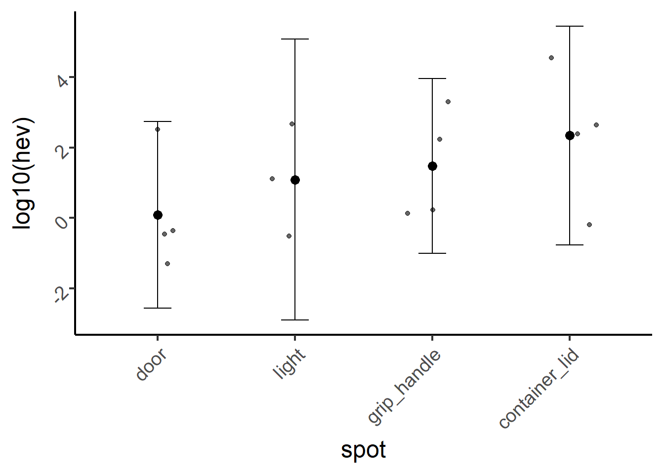
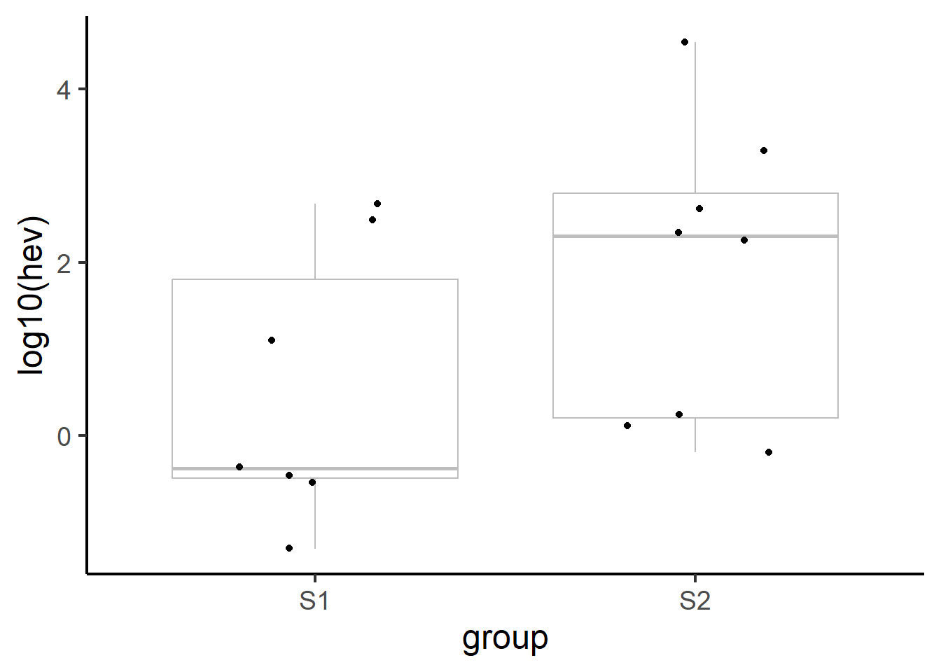
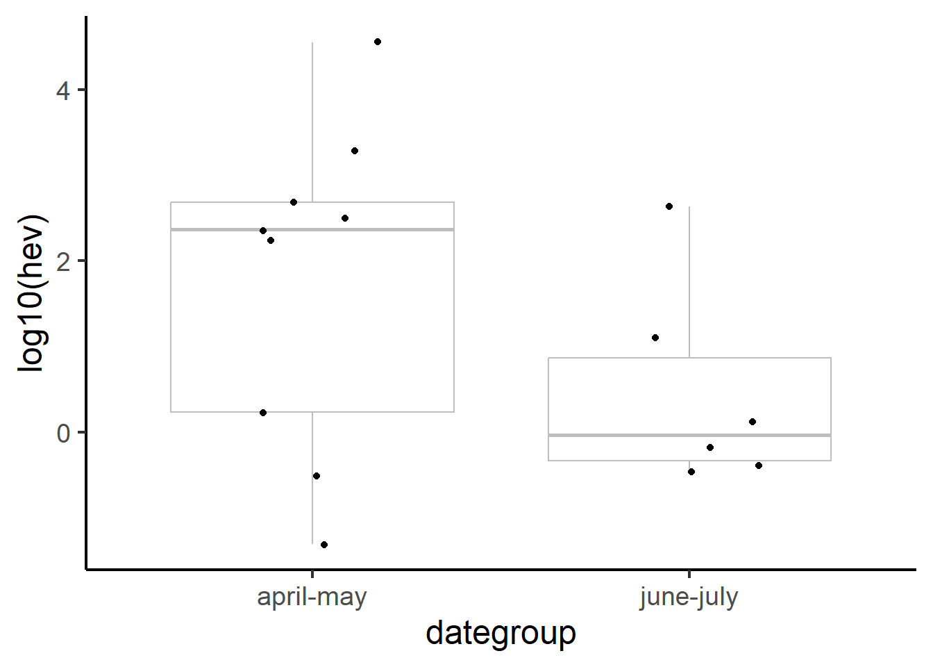
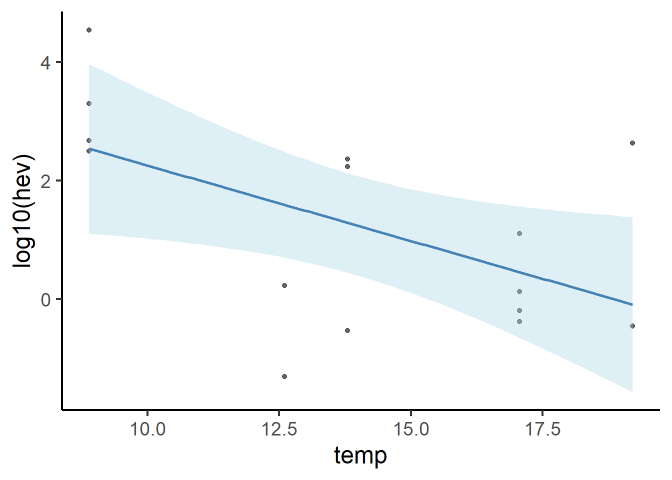
Frequency of hand-to-surface contacts per work day (“jornada laboral”) (events/day), \(f_{conv|surf} \sim\) Uniform \((a, b)\) (from RiskHEV.xlsx$3-Dades_gomets):
spot
a
b
light
6
8
door
2
20
container_lid
0
4
grip_handle
0
4
To integrate different spots within S1 we may use a mixture between both distributions (also for HEV concentrations).
Viral transfer efficiency from surface to bare hands (%), \(TE_{surf|hand} \sim\) Normal \((\mu = 37, \sigma = 16)\)(Lopez et al. 2013).
Viral transfer efficiency from hands to mouth (%), \(TE_{hand|mouth} = 34\)(Rusin et al. 2002).
Frequency of hand-to-mouth contacts (events/hour), \(f_{cont|mouth}\). The distribution can be learnt from the data of Wilson et al. (2021), available at https://doi.org/10.5518/798 (data_face_contact.csv).
Distribution with \(\mu\simeq\) 2.92 and \(\sigma \simeq\) 2.54.
We thought of not including \(n_{hours}\) as we consider daily doses. However, \(f_{cont|mouth}\) is given in events/hour. Q3. So we need to define \(n_{hours}\). We can use \(U(4,6)\) as in Itarte et al. (2024) .
\[ P_{inf}(d|\alpha,\beta) = 1 - \left(1 + \frac{d}{\beta} \right)^{-\alpha} \] This approximation is valid when \(\alpha << \beta\) and \(\beta >> 1\)(Haas et al. 2014).
Reparametrization based on \(N_{50}\)
\[ P_{inf}(d |\alpha, N_{50}) = 1 - \left ( 1 + (2^{1/\alpha}-1)\cdot \frac{d}{N_{50}}\right ) ^{-\alpha}\] where \(\beta = \frac{N_{50}}{2^{1/\alpha}-1}\). A good description of the Beta-Poisson model is provided in Teunis et al. (2000).
Parameter estimation
Parameters derived for HEV from chimpanzee data via MLE in Ruchusatsawat et al. (2022):
95% CI for both parameters are shown in Figs. 2-3, but data (to the best of my knowledge) is not provided.
Wilkins et al. (2025) refers to Müller et al. (2017) and AFSSA (2009) and suggests to use \(N_{50} = 10^{5.5}\) instead (based on consumption of pork-derived products). It seems more realistic to use this value in our scenario.
Q4. In Itarte et al. (2024) we have an equation (eq. 4) to compute \(P_{ill}\) (probability of illness) from \(P_{inf}\) (probability of infection), but for HEV we do not have such equation (we lack the parameter estimates). In Ruchusatsawat et al. (2022), they use a similar strategy (eqs. 6 and 11). We may be able to use this, but I am not sure whether it would be equivalent. Discuss in person.
QMRA test (1)
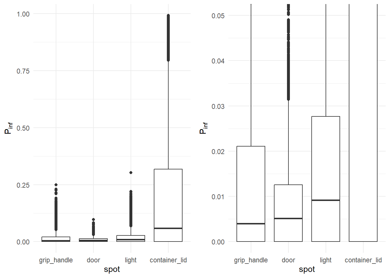
Considering uniform distributions for \(C_{HEV}\).
Haas, C. et al. 2014. Quantitative Microbial Risk Assessment: Second Edition. Quantitative Microbial Risk Assessment: Second Edition. Vol. 9781118145296. Wiley Blackwell. https://doi.org/10.1002/9781118910030.
Itarte, M. et al. 2024. “Assessing environmental exposure to viruses in wastewater treatment plant and swine farm scenarios with next-generation sequencing and occupational risk approaches.”International Journal of Hygiene and Environmental Health 259 (June): 114360. https://doi.org/10.1016/J.IJHEH.2024.114360.
Lopez, G. U. et al. 2013. “Transfer Efficiency of Bacteria and Viruses from Porous and Nonporous Fomites to Fingers under Different Relative Humidity Conditions.”Applied and Environmental Microbiology 79 (18): 5728–34. https://doi.org/10.1128/AEM.01030-13.
McBride, G. B. et al. 2013. “Discharge-based QMRA for estimation of public health risks from exposure to stormwater-borne pathogens in recreational waters in the United States.”Water Research 47 (14): 5282–97. https://doi.org/10.1016/J.WATRES.2013.06.001.
Müller, A. et al. 2017. “Assessment of the risk of foodborne transmission and burden of hepatitis E in Switzerland.”International Journal of Food Microbiology 242 (February): 107–15. https://doi.org/10.1016/J.IJFOODMICRO.2016.11.018.
Ruchusatsawat, K. et al. 2022. “Quantitative Risk Assessments of Hepatitis A Virus and Hepatitis E Virus from Raw Oyster Consumption.”Risk Analysis 42 (5): 953–65. https://doi.org/10.1111/RISA.13832.
Rusin, P. et al. 2002. “Comparative surface‐to‐hand and fingertip‐to‐mouth transfer efficiency of gram‐positive bacteria, gram‐negative bacteria, and phage.”Journal of Applied Microbiology 93 (4): 585–92. https://doi.org/10.1046/J.1365-2672.2002.01734.X.
Teunis, P. et al. 2000. “The Beta Poisson Dose-Response Model Is Not a Single-Hit Model.”Risk Analysis 20 (4): 513–20. https://doi.org/10.1111/0272-4332.204048.
Wilkins, N. et al. 2025. “A farm-to-consumption quantitative microbiological risk assessment for hepatitis E in pigs.”Risk Analysis, 1–16. https://doi.org/10.1111/RISA.70035.
Wilson, A. M. et al. 2021. “Frequency of hand-to-head, -mouth, -eyes, and -nose contacts for adults and children during eating and non-eating macro-activities.”Journal of Exposure Science & Environmental Epidemiology 2020 31:1 31 (1): 34–44. https://doi.org/10.1038/s41370-020-0249-8.
Source Code
---title: "QMRA (HEV)"author: "Diego Garrido"date: "`r format(Sys.time(), '%d %B, %Y')`"format: html: code-fold: true code-tools: trueexecute: echo: false tidy: true warning: false message: falseknitr: opts_chunk: fig.align: centerbibliography: refs.bib---```{r}library(dplyr)library(ggplot2)library(cowplot)library(fitdistrplus)```## Data### Original datasetFrom `RiskHEV.xlsx$3-Dades_gomets` and `temperaturesmostreig gomets.xlsx`.<details><summary>Details</summary>```{r, echo = T}tb = data.frame( spot = c( rep(c("llum", "porta", "bossa identificativa (pinça)", "contenidor manec ferro", "contenidor interior"), 4), "llum", "porta", "cinta contenidor","int", "ext-contenidor interior"), date = as.Date(c( rep("04/24/2024", 5), rep("05/08/2024", 5), rep("05/23/2024", 5), rep("06/05/2024", 5), rep("06/24/2024", 3), rep("07/15/2024", 2) ), format = "%m/%d/%Y"), temp = c( rep(8.89, 5), rep(12.6, 5), rep(13.8, 5), rep(17.06, 5), rep(19.21, 3), rep(22.2, 2) ), hev = c( 4.77E+02, 3.14E+02, NA, 2.00E+03, 3.51E+04, NA, 4.90E-02, NA, 1.70E+00, NA, 2.97E-01, NA, NA, 1.74E+02, 2.31E+02, 1.29E+01, 4.17E-01, 1.20E-01, 1.34E+00, 6.40E-01, NA, 3.51E-01, 4.30E+02, NA, NA ))``````{r}knitr::kable(format(tb, scientific = F))```</details>### Data preprocessing- Remove spot: "*bossa identificativa (pinça)*"- Rename spots in english- Make groups: `S1`: "*door*" + "*light*"; `S2`: "*container_lid*" + "*grip_handle*"- Add helper columns: `group`, `datenum` (days from 2024-04-01), `dategroup````{r, echo = T}tb %<>% filter(spot != "bossa identificativa (pinça)") %>% mutate( spot = case_when( spot == "porta" ~ "door", spot == "llum" ~ "light", spot %in% c("cinta contenidor", "ext-contenidor interior", "contenidor interior", "int") ~ "container_lid", spot == "contenidor manec ferro" ~ "grip_handle", TRUE ~ spot ), group= case_when( spot %in% c("door", "light") ~ "S1", spot %in% c("container_lid", "grip_handle") ~ "S2" ), datenum = as.numeric(date - as.Date("2024-04-24")), dategroup = ifelse(datenum <= 29, "april-may", "june-july") )``````{r}knitr::kable(format(tb, scientific = F))```### Descriptive stats```{r, echo = T}set.seed(123)# ggplot(tb[!is.na(tb$hev), ], aes(y = log10(hev), x = spot)) +# geom_boxplot(col = "gray", outlier.size = 0) +# geom_jitter(width = 0.2) +# theme_classic(base_size = 18) +# theme(axis.text = element_text(angle = 45, hjust = 1))tbs <- tb %>% filter(!is.na(hev)) %>% mutate(spot = forcats::fct_reorder(spot, hev, .fun = mean))ggplot(tbs[!is.na(tbs$hev), ], aes(x = spot, y = log10(hev))) + stat_summary(fun = mean, geom = "point", size = 3) + stat_summary( fun.data = mean_cl_normal, geom = "errorbar", width = 0.2 ) + geom_jitter(width = 0.2, alpha = 0.6) + theme_classic(base_size = 18) + theme(axis.text = element_text(angle = 45, hjust = 1))ggplot(tb[!is.na(tb$hev), ], aes(y = log10(hev), x = group)) + geom_boxplot(col = "gray", outlier.size = 0) + geom_jitter(width = 0.2) + theme_classic(base_size = 18) ggplot(tb[!is.na(tb$hev), ], aes(y = log10(hev), x = dategroup)) + geom_boxplot(col = "gray", outlier.size = 0) + geom_jitter(width = 0.2) + theme_classic(base_size = 18)``````{r, echo = T}# fisher.test(with(tb, table(dategroup, is.na(hev))))# ggplot(tb[!is.na(tb$hev), ], aes(x = datenum, y = log10(hev))) +# geom_point(alpha = 0.6) + # geom_smooth(method = "lm", se = TRUE, # linewidth = 1, colour = "steelblue",# fill = "lightblue") +# theme_classic(base_size = 18) # # lm.fit <- lm(log10(hev)~datenum, data = tb)# # plot(lm.fit)# summary(lm.fit)ggplot(tb[!is.na(tb$hev), ], aes(x = temp, y = log10(hev))) + geom_point(alpha = 0.6) + geom_smooth(method = "lm", se = TRUE, linewidth = 1, colour = "steelblue", fill = "lightblue") + theme_classic(base_size = 18) lm.fit <- lm(log10(hev)~datenum, data = tb)# plot(lm.fit)summary(lm.fit)```- `NA`s substituted by 0:```{r, echo = T}tb2 = tbtb2$hev[is.na(tb2$hev)] = 1 # then log(1) = 0# ggplot(tb2, aes(x = datenum, y = log10(hev))) +# geom_point(alpha = 0.6) + # geom_smooth(method = "lm", se = TRUE,# linewidth = 1, colour = "steelblue",# fill = "lightblue") +# theme_classic(base_size = 18)# # lm.fit2 <- lm(log10(hev)~datenum, data = tb2)# # plot(lm.fit)# summary(lm.fit2)ggplot(tb2, aes(x = temp, y = log10(hev))) + geom_point(alpha = 0.6) + geom_smooth(method = "lm", se = TRUE, linewidth = 1, colour = "steelblue", fill = "lightblue") + theme_classic(base_size = 18)lm.fit2 <- lm(log10(hev)~datenum, data = tb2)# plot(lm.fit)summary(lm.fit2)```## Exposure assesment### Surface model$$d = C_{HEV} \times \frac{f_{conv}}{r_{eff}} \times f_{conv|surf} \times TE_{surf|hand} \times TE_{hand|mouth} \times f_{cont|mouth} \times n_{hours}$$- Concentration of HEV (surface, CG/cm$^2$), $C_{HEV} \sim$ Lognormal$(\mu, \sigma)$. We consider left-censored data.<div style="margin-left: 2em;">- Group `S1`:<div style="margin-left: 4em;">```{r, echo = T}tbs1 = subset(tb, group == "S1")tbs1cens = data.frame(left = tbs1$hev, right = tbs1$hev)tbs1cens$right[is.na(tbs1cens$right)] = min(tbs1cens$right, na.rm = T)fit1 = fitdistcens(tbs1cens, distr = "lnorm")fit1```<mark>**Q1**. Detection limit is 4.56 GC/cm\^2. How is it possible that there are values below?</mark></div>- Group `S2`:<div style="margin-left: 4em;">```{r, echo = T}tbs2 = subset(tb, group == "S2")tbs2cens = data.frame(left = tbs2$hev, right = tbs2$hev)tbs2cens$right[is.na(tbs2cens$right)] = min(tbs2cens$right, na.rm = T)fit2 = fitdistcens(tbs2cens, distr = "lnorm")fit2```</div></div><div style="margin-left: 2em;"><mark> **Q2**. Maybe we should do $U(0, max)$ for each spot. </mark></div>- Conversion factor (TCID50/GC), $f_{conv} = \frac{1}{700}$ [@McBride2013].- Recovery efficiency (%), $r_{eff} = 7.3$ [@Itarte2024].- Frequency of hand-to-surface contacts per work day ("*jornada laboral*") (events/day), $f_{conv|surf} \sim$ Uniform $(a, b)$ (from `RiskHEV.xlsx$3-Dades_gomets`):<div style="margin-left: 2em;">```{r}# removed "bossa identificativa (pinça)"contact =data.frame(spot =c("light", "door", "container_lid","grip_handle"),a =c(6, 2, 0, 0),b =c(8, 20, 4, 4))knitr::kable(contact)```To integrate different spots within `S1` we may use a mixture between both distributions (also for HEV concentrations).```{r}which_dist <-sample(c(1, 2), size =1, prob =c(0.5, 0.5)) # shared for HEV concentrationsmpl =floor(ifelse(which_dist ==1, sample(6:8, size =1), sample(2:20, size =1)))```</diV>- Viral transfer efficiency from surface to bare hands (%), $TE_{surf|hand} \sim$ Normal $(\mu = 37, \sigma = 16)$ [@Lopez2013].- Viral transfer efficiency from hands to mouth (%), $TE_{hand|mouth} = 34$ [@Rusin2002].- Frequency of hand-to-mouth contacts (events/hour), $f_{cont|mouth}$. The distribution can be learnt from the data of @Wilson2021, available at https://doi.org/10.5518/798 ([data_face_contact.csv](https://archive.researchdata.leeds.ac.uk/680/1/data_face_contact.csv)).<div style="margin-left: 2em;">```{r, echo = T}data_face_contact <- read.csv(url("https://archive.researchdata.leeds.ac.uk/680/1/data_face_contact.csv"))f_contmouth = subset(data_face_contact, eatonly == "Non-eating" & age == "adult" & contactarea == "mouth")$frequencypmf_contmouth <- table(f_contmouth) / length(f_contmouth)# sum(pmf_contmouth)# Non-parametric samplingset.seed(123)sampl <- sample(as.numeric(names(pmf_contmouth)), size = 1e6, replace = TRUE, prob = pmf_contmouth)```Distribution with $\mu\simeq$ `r round(mean(sampl),2)` and $\sigma \simeq$ `r round(sd(sampl),2)`.</div>- We thought of not including $n_{hours}$ as we consider daily doses. However, $f_{cont|mouth}$ is given in events/hour. <mark> **Q3.** So we need to define $n_{hours}$. We can use $U(4,6)$ as in @Itarte2024 </mark>.## Dose-response model (Beta-Poisson)### Exact model$$ P_{inf}(d|\alpha,\beta) = 1 - {}_1F_1\left( \alpha, \alpha + \beta, -d \right) $$### Approximation$$ P_{inf}(d|\alpha,\beta) = 1 - \left(1 + \frac{d}{\beta} \right)^{-\alpha} $$ This approximation is valid when $\alpha << \beta$ and $\beta >> 1$ [@Haas2014].### Reparametrization based on $N_{50}$$$ P_{inf}(d |\alpha, N_{50}) = 1 - \left ( 1 + (2^{1/\alpha}-1)\cdot \frac{d}{N_{50}}\right ) ^{-\alpha}$$ where $\beta = \frac{N_{50}}{2^{1/\alpha}-1}$. A good description of the Beta-Poisson model is provided in @Teunis2000.## Parameter estimationParameters derived for HEV from chimpanzee data via MLE in @Ruchusatsawat2022:- $\alpha = 216.89$- $N_{50} = 3.03 \cdot 10^7$ (intravenous inoculation)95% CI for both parameters are shown in Figs. 2-3, but data (to the best of my knowledge) is not provided.@Wilkins2025 refers to @Muller2017 and @AFFSA2009 and suggests to use $N_{50} = 10^{5.5}$ instead (based on consumption of pork-derived products). It seems more realistic to use this value in our scenario.<mark>**Q4**. In @Itarte2024 we have an equation (eq. 4) to compute $P_{ill}$ (probability of illness) from $P_{inf}$ (probability of infection), but for HEV we do not have such equation (we lack the parameter estimates). In @Ruchusatsawat2022, they use a similar strategy (eqs. 6 and 11). We may be able to use this, but I am not sure whether it would be equivalent. Discuss in person.</mark>## QMRA test (1)Considering uniform distributions for $C_{HEV}$.```{r, echo = T}set.seed(123)nsim = 1e4res = list()spots = c("door", "light", "grip_handle", "container_lid")for (where in spots){ C_HEV = runif(n = nsim, ifelse(is.na(min(subset(tb, spot==where)$hev)), 0, min(subset(tb, spot==where)$hev)), max(subset(tb, spot==where)$hev, na.rm = T)) f_conv = 1/700 r_eff = 7.3 range_vals <- switch(where, door = 6:8, light = 2:20, grip_handle = 0:4, container_lid = 0:4 ) f_conv_surf = sample(range_vals, replace = T, size = nsim) TE_surf_hand = rnorm(n = nsim, mean = 37, sd = 6) TE_hand_mouth = 34 f_cont_mouth = sample(as.numeric(names(pmf_contmouth)), replace = T, size = nsim, prob = pmf_contmouth) n_hours = sample(4:6, size = nsim, replace = T) d = C_HEV*f_conv/r_eff*f_conv_surf*TE_surf_hand*TE_hand_mouth*f_cont_mouth*n_hours alpha = 216.89 N50 = 10^5.5 P_inf = 1 - (1 + (2^(1/alpha) - 1)*d/N50)^(-alpha) res[[where]] = P_inf}# For plottingdf = data.frame( spot = rep(spots, times = lengths(res)), probs = unlist(res, use.names = FALSE))medians <- tapply(df$probs, df$spot, median)df$spot <- factor(df$spot, levels = names(sort(medians)))pl = ggplot(df, aes(x = spot, y = probs)) + geom_boxplot() + theme_minimal() + labs(y = expression(P[inf]))plz = ggplot(df, aes(x = spot, y = probs)) + geom_boxplot() + theme_minimal() + coord_cartesian(ylim = c(0,0.05)) + labs(y = expression(P[inf]))plot_grid(pl, plz)```## References::: {#refs}:::